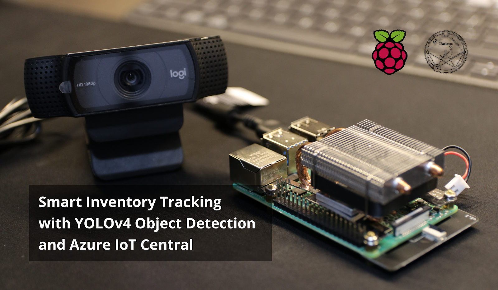
Machine Learning Powered Inventory Tracking with Raspberry Pi

In today’s tutorial, I will show you how to create a smart inventory tracker using object detection, powered by deep learning, with just a Raspberry Pi 4 and a camera. We will apply transfer learning on the YOLOv4 tiny model to identify custom objects, then use a simple python script to parse the model’s output to produce a count of each object. Finally, we will also integrate the application with Azure IoT Central so that we can monitor our inventory remotely and conveniently.

Project Overview

Have you ever passed by a grocery store but found yourself unsure of whether you needed to get that extra carton of milk? Well, what if there was some way to have eyes on the inside of our fridge to update us with that information? Today, with machine learning and IoT infrastructures, we are going to turn that convenience into reality.

To summarize, we want to create two key features in our project. First, to automatically count the items in our fridge. Then, to be able to access the data remotely when we need it. Before we begin, let’s take a look at a short video demonstration below.

Machine Learning: Image Classification vs Object Detection

Object recognition tasks like image classification and object detection are both performed with deep neural networks, but it is meaningful to differentiate between the two. In image classification, our input is an image that contains a single class. For example, we might have a photo of a single cat, or a dog, that we want the model to classify as a single output.

In object detection, however, we want the model to not only identify multiple objects, but to also locate all the instances of each class present in a photo. Indeed, as opposed to classification, we will now be able to count the number of each type of object present in the frame – just what we need for this project!

For more information, Jason Brownlee’s article is a great introduction to the different types of computer vision tasks.

What is Transfer Learning?

Because computer vision tasks in general are considered complex tasks, it can take days to train a functional model even on a powerful GPU. Fortunately, as long as we have both the architecture and the weights, anyone can easily implement existing models that have already been trained.

However, what if we want to train the model to recognise other things? After all, it’d be a farfetch to expect these models to naturally be great at recognising our household’s specific choice of grocery products. In this case, we don’t have to train a new model from scratch. Instead, we can apply transfer learning.

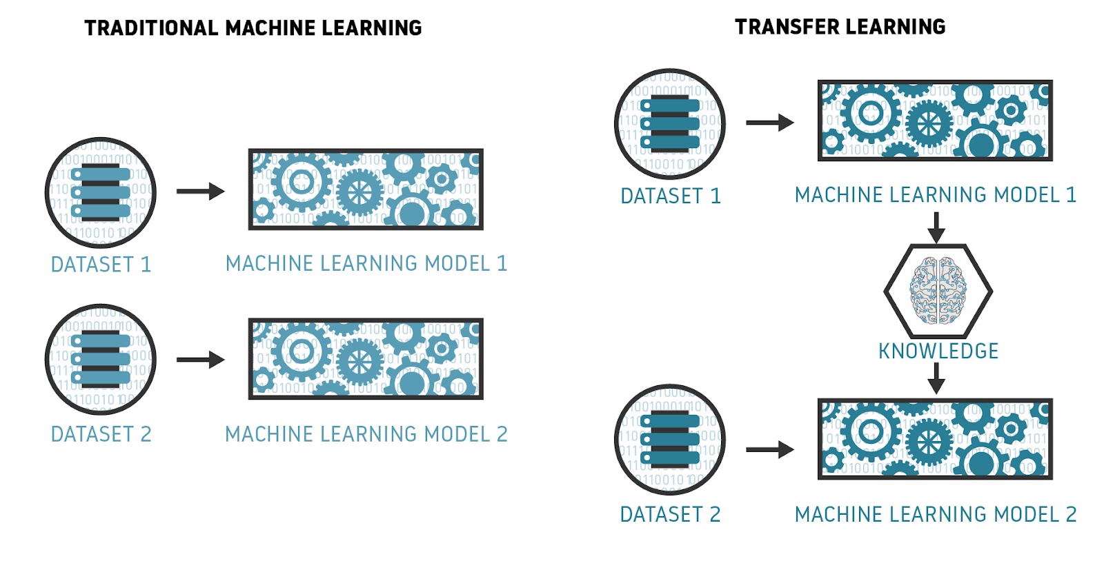
Transfer learning is a technique where we utilise a pretrained model, and train it with a new dataset with the objective of accomplishing a similar task. It allows us to achieve higher performance in our models with less data, while still drastically reducing the amount of time and resources required for training. Today, we will perform transfer learning with YOLOv4 Tiny.

What is YOLO?

YOLO, which stands for You Only Look Once, is a state of the art neural network machine learning framework for object detection. When its first paper was released in 2015, it beat out the other models in inferencing speed, allowing for real time object detection at some expense of accuracy. Today, work on YOLO has continued under different parties to bring improvements in accuracy while retaining low latency.

For today’s project, we are using the 4th version, YOLOv4. More specifically, we will be using the tiny version of YOLOv4, which has a smaller network size. While we do sacrifice some accuracy with a smaller model, this brings a reduction in the computing power requirements, allowing the model to be run with decent performance on an edge device like our Raspberry Pi.

Prepare Your Custom Dataset

As our first step to train our custom model, we will have to build our dataset by gathering photos of the items that we want to detect. You’ll want at least 50 images of each class. In my project, I decided to count the number of milk cartons, eggs, and yoghurt packets, so my dataset should end up with at least 150 images in total.

Here are some tips when collecting your dataset.

In general, capture images with a variety of lighting conditions and camera angles, and of the objects in different orientations to create a more robust dataset.
For objects that usually exist in multiples, such as eggs, be sure to include individual images as well as others in groups.
If you often stack some objects, like milk cartons, you’ll want to include several images where they are stacked so that our model can learn accordingly.

Label Dataset with labelImg

There are many open source tools for labelling images for computer vision projects. I’ve decided to go with labelImg. It’s free, open source, and can be easily installed and run with the following two commands.

pip3 install labelImg
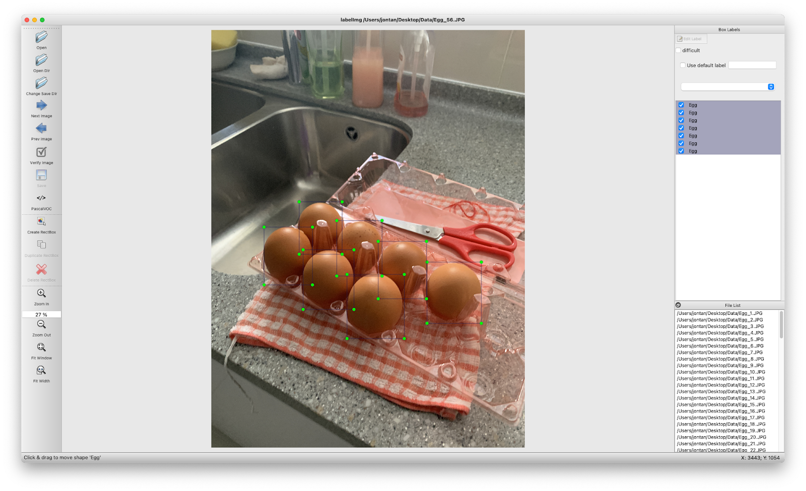
labelImg

The GUI (graphical user interface) should open up and you can get to work labelling your images! Use Open Dir on the left pane to select the folder that your images are in. When they’re loaded in, use W and click-drag to begin drawing bounding boxes around your objects.

Before saving each file, ensure that the export format is Pascal VOC, which should write to an xml file of the same name as the image. When you’re done, you should end up with a folder with a bunch of images and xml files, like I have below.

Process Labelled Data with RoboFlow

We’ll first use Roboflow’s platform to augment our images. While we could do this ourselves programmatically, Roboflow offers some conveniences for later on. Augmentation is a technique in computer vision data processing where we apply transformations to our images through flipping, rotating, skewing, recolouring etc.

This is very powerful, since each transformation essentially yields one new photo. If we create three augmented versions of each training sample, we would have 4 times the number of total samples! Besides, who has the patience to label 200 photos per class by hand?

*Source: Valentina Alto on Analytics Vidhya*

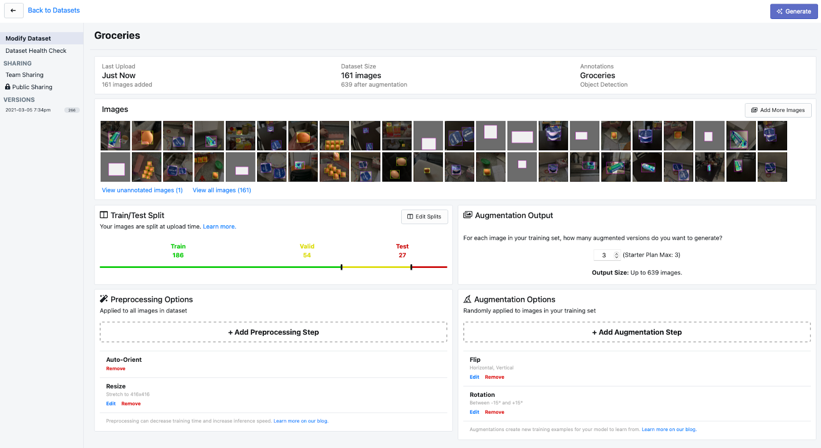
To get started, first sign up for a Roboflow account here. The free account has some limits, but will be sufficient for our project today. Once you’re logged in, create a new dataset for Object Detection (Bounding Box). You can name it whatever you like. I named mine “Groceries”, since it might be useful to generalise this dataset in the future.

Then, drag and drop your image and xml files to upload them. Select “Finish Uploading” when you’re done, and let Roboflow split the data for you. Under Augmentation Options, add Flip Horizontal and Vertical, along with Rotation -15, +15. Under preprocessing, Auto-Orient and Resize should have been done automatically. If not, you can reference the screen capture that I have below.

On the top right corner, click on Generate. Once done, select “YOLO Darknet” format and “show download code”. Then, you will be greeted with a !curl command. Save this for use in the later part of our tutorial.

Transfer Learning on Google Colab

Now it’s time to perform transfer learning! This section is based on Roboflow’s tutorial and its accompanying Colab notebook, which performs transfer learning with a blood cell dataset.

For this project, I made some minor changes to Roboflow’s notebook so that the code will run with the GPU provided to free Colab users by default. First save a copy of my notebook to your Google Drive so that you can make edits.

In your copy, navigate to Edit > Notebook Settings, and ensure that GPU is selected for hardware accelerator. Unless your GPU architecture is different for some reason, the only other change you have to make will be the first cell in the “Set up Custom Dataset for YOLOv4” section. Replace the last line with the curl command from the previous section.

# Paste your link here
%cd /content/darknet
!curl -L <YOUR LINK> > roboflow.zip; unzip roboflow.zip; rm roboflow.zip

For those curious, this notebook essentially automates the changes that we would need to make to the YOLOv4 Tiny architecture according to our dataset. The original step by step instructions can be found here, but they are long and can be confusing for beginners.

Now, proceed to run the cells one by one. The training will take awhile, but before you head off for a break, take note that a reset of the Google Colab runtime will erase all the files created from the session. Yes – this includes the weights of the model!

Important! Once the training block is complete, be sure to grab the following before the runtime hits a timeout.

Save the best weights from content/darknet/backup/custom-yolov4-tiny-detector_best.weights
Extract custom-yolov4-tiny-detector.cfg from content/darknet/cfg

The remaining three cells can be used to test our model on our test data. You can repeatedly run the last cell to pull a different random photo for the model to infer on.

ML Inferencing on the Edge with Raspberry Pi

Now that we have our custom YOLOv4 tiny model, we can proceed to test it on our Raspberry Pi. To do that, we first have to set up our environment. Note: This tutorial uses Raspberry Pi OS.

Step 1: Clone AlexeyAB’s darknet repository on your Raspberry Pi and compile with make.

git clone https://github.com/AlexeyAB/darknet
cd darknet
make

Step 2: Edit the coco.names file under ./darknet/data/coco.names. Using any text editor, replace the classes inside this file with your custom classes. In my case, it’s the following.

Egg
Milk
Yoghurt

Step 3: Place your saved weights from the Colab notebook inside the darknet/backup folder, and the custom-yolov4-tiny-detector.cfg inside the darknet/cfg folder.

Step 4: Place a test image of your choice named “test.jpg” in the darknet folder, and run the following command to test the model.

./darknet detect cfg/custom-yolov4-tiny-detector.cfg backup/custom-yolov4-tiny-detector_best.weights test.jpg -dont-show

The results should then be shown in the command line interface. Great! You’ll notice that the time it takes for running the inference is quite long – over 7 seconds. Fortunately, since there’s no need to update the fridge’s inventory so frequently, this won’t be an issue.

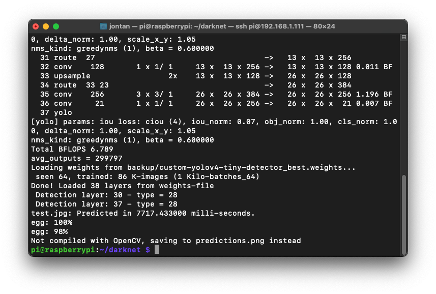
A predictions.png file should also be generated in the darknet folder, so you can see the bounding boxes generated around each item.

Deploy on Microsoft Azure IoT Central

Of course, what we’ve done so far wouldn’t be very useful if we couldn’t access this data remotely. The next step of our project is to create an Azure IoT Central Application where we will periodically send our inventory status, so that we can monitor it remotely. Before proceeding, create a free Microsoft Azure account here.

Step 1: Create an Azure IoT Central application

Head over to Azure IoT Central. Scroll down and select Create a custom app. You will be prompted to log in before being shown the screen below. Choose an application name and URL, and leave the Application template as Custom application. Under pricing plan, select free for now. Then, proceed to create your application.

Step 2: Add a Device Template

Using the sidebar, navigate to Device template, then click on +New. From there, select IoT device then Next: Customize. From here, select a device template name – I went with “RaspberryPi”. Then, proceed to create the template.

Step 3: Add Interface & Capabilities to Device Template

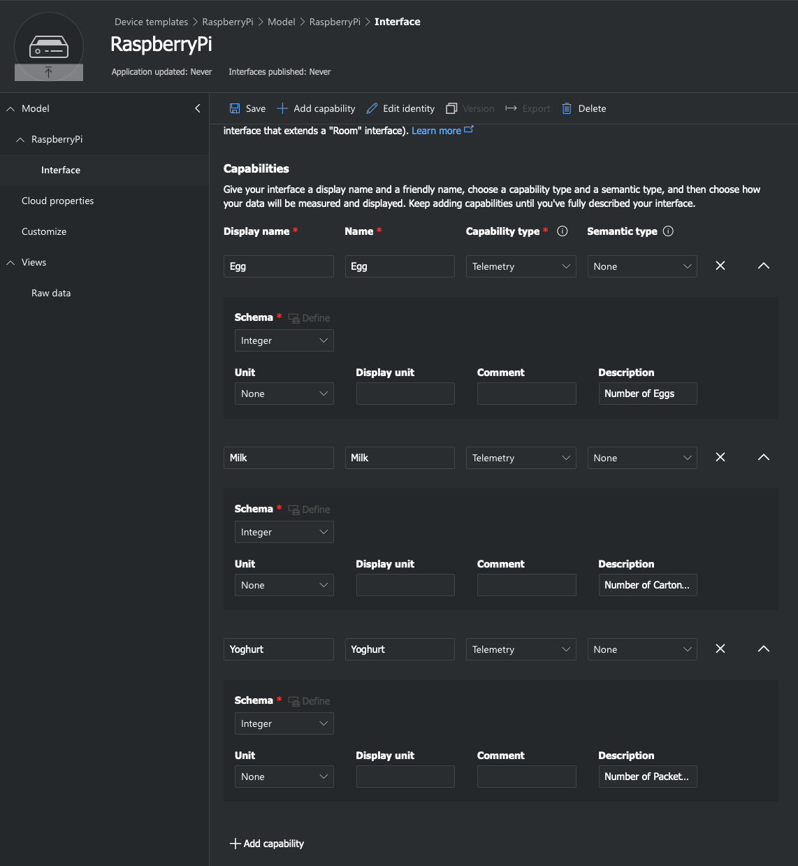
Following the previous step, you should have been taken automatically to your new device template. Select Custom model, then Add an inherited interface. Once again, select custom.

After that, you will need to add capabilities to your interface according to the items that you are keeping track of. Be sure that these are the right parameters that you want, as they can’t be changed after we publish our device template. Click on save, but do not publish for now.

Step 4: Set Up Device View

To visualise our data nicely on our Azure IoT Central application, we have to set up our device view. Navigate to Views on the device panel and select Visualizing the device.

Following this, under the Edit view pane, click on Select a Telemetry. Choose your first item and click Add tile. The tile should appear on your dashboard preview on the right. For each of the tiles, change their display value to “last known value”.

I added three tiles for a total of three items, ending up with the dashboard shown below. Once you are satisfied with your settings, click on Publish at the top of the page.

Step 5: Create a Device

Now, we have to create a device. Navigate to Devices and click on + New. Enter a device name of your choice, and remember to select the device template that you created previously. I went with “Rpi”.

Click into the device you just created. You should see the dashboard that you set up earlier, but without any data shown. We’ll fix that in a moment by getting our Raspberry Pi to send some data to our Azure IoT Central application. Click “Connect” on the top right of the screen and a window should pop up.

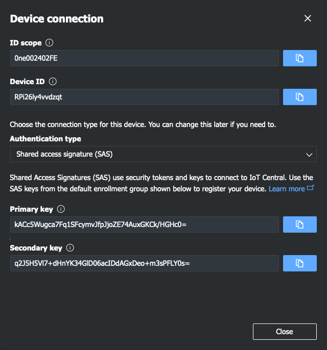
Step 6: Generate Connection Key

Open this Azure IoT Central Connection String Generator in a new browser window. Fill the blanks in with the corresponding data from the window above. Take note that “Device Key” refers to the primary key. Finally, record down the connection string that is generated for later.

Step 7: Set Up Raspberry Pi for Azure IoT

As a final step, run the following command on your Raspberry Pi CLI to install the related packages for Azure IoT.

sudo pip3 install azure-iot-device azure-iot-hub azure-iothub-service-client azure-iothub-device-client

Running Through the Complete Workflow

We’ve been working with bits and pieces so far, but it’s finally time to put it all together to create our machine learning powered Smart Fridge Inventory Tracker. Before following with these steps, first visit my Github repository here and download the files as a ZIP. Place img.txt and parseSendData.py into your darknet folder.

1. Take a Photo

First, we take a photo with the camera attached to the Raspberry Pi using the command … . The file is saved to the darknet folder as img.jpg.

For the Raspberry Pi Camera module, use the following. Ensure that the camera is enabled via raspi-config > Interface first.

raspistill -o /darknet/img.jpg

If you are using a USB webcam like me, first install the fswebcam package, then we can take photos in a similar manner. The second command takes a photo and writes it to the darknet folder as img.jpg with a specific delay, frameskip and resolution. You can adjust them to your preference.

sudo apt-get install fswebcam
fswebcam -D 2 -S 20 -r 1920x1080 --no-banner darknet/img.jpg

2. Run & Record the Inference Results

To parse the data and send it to Azure IoT Central, we will need to get the model’s output in a text file. We use the following command to read in the files listed in img.txt (only img.jpg), perform object detection, and write the output to result.txt.

./darknet detector test cfg/coco.data cfg/custom-yolov4-tiny-detector.cfg backup/custom-yolov4-tiny-detector_best.weights -dont_show -ext_output < img.txt > result.txt

3. Parse & Send Data to Azure IoT Central

Now, open parseSendData.py. This is a simple Python script that will parse the result.txt file, count the instances of each class and then send it to Azure IoT Central. First, replace the CONNECTION_STRING with the one you obtained in Step 12 of the previous section.

CONNECTION_STRING = <Replace with your own string>

Then, update the dictionary by replacing the keys with your item classes. Please note that you must match the string for each class according to what you have written in the coco.data file previously. Otherwise, you will encounter a key error.

Now, run the python script through your command line with the following:

python3 <yourpath>/parseSendData.py

If all goes well, you should see something similar to the following output, and the script will complete without errors.

Attempting to Send Messages to Azure IoT
Sending message: {'Egg': 6, 'Milk': 1, 'Yoghurt': 2}
Message Sent

Head back to your device view on Azure IoT Central. The numbers should show up in a few moments!

Automate the Workflow

The last step that we need to do is to automate the entire process of the previous section with a bash script. Fortunately, we can use cron to schedule the entire process to run automatically at half-an-hour intervals on our Raspberry Pi.

First, we create a bash script titled “workflow.sh” as follows in our darknet folder. A bash script is essentially a list of console commands that can be run together in a group, so they don’t have to be run individually. Later on, we will use cron to execute this script automatically.

fswebcam -D 2 -S 20 -r 1920x1080 --no-banner img.jpg
./darknet detector test cfg/coco.data cfg/custom-yolov4-tiny-detector.cfg backup/custom-yolov4-tiny-detector_best.weights -dont_show -ext_output < img.txt > result.txt
python3 parseSendData.py

Then, we make the script executable by running the following command. Make sure that your present working directory is the darknet folder, where the script is located.

chmod +x workflow.sh

Now, if you run the script, you should see the entire workflow occur automatically and consecutively in your terminal output. Our program will take the photo, run the model, parse the data and upload it to Azure IoT Central with just one execution. Neat!

To schedule the execution of this script with cron, first open the crontab editor by running the command below. Cron is preinstalled with Raspberry Pi OS.

crontab -e

You will be prompted to select an editor. If you don’t know which to choose, pick the simple nano editor (the first option). Then, a file will open in your command line. We have to add our scheduled command to this file for it to run automatically. At the bottom of the file, add the following.

*/30 * * * * /home/pi/darknet/workflow.sh

And that’s it! Get your Raspberry Pi and camera in position, and you should see the data flow into your Azure IoT Central application at the next half-hour mark.

Conclusion

Thanks for reading! I hope this article was helpful in the creation of your smart inventory tracking project. It’s amazing how accessible it has become to build a machine learning application for personal use. With IoT and cloud integration, these applications are even more useful in meeting practical needs.

For more projects involving machine learning on the edge, feel free to have a look at the below:

About Author

Jonathan Tan

See author's posts

Tags: AI, Computer Vision, Edge AI, Edge Computing, object detection, Raspberry Pi, Raspberry Pi 4, raspberry pi camera, Raspberry Pi projects

M	T	W	T	F	S	S
1	2	3	4	5	6	7
8	9	10	11	12	13	14
15	16	17	18	19	20	21
22	23	24	25	26	27	28
29	30	31